|
ME 405 Portfolio
|


|
|
ME 405 Portfolio
|
|
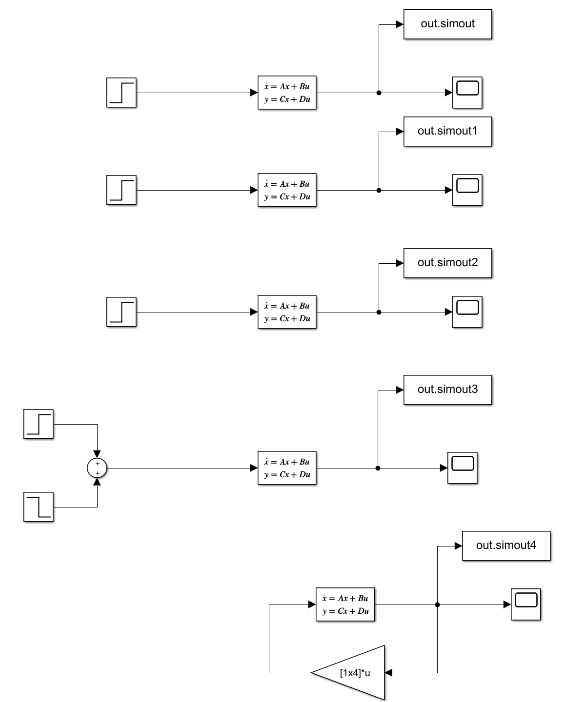
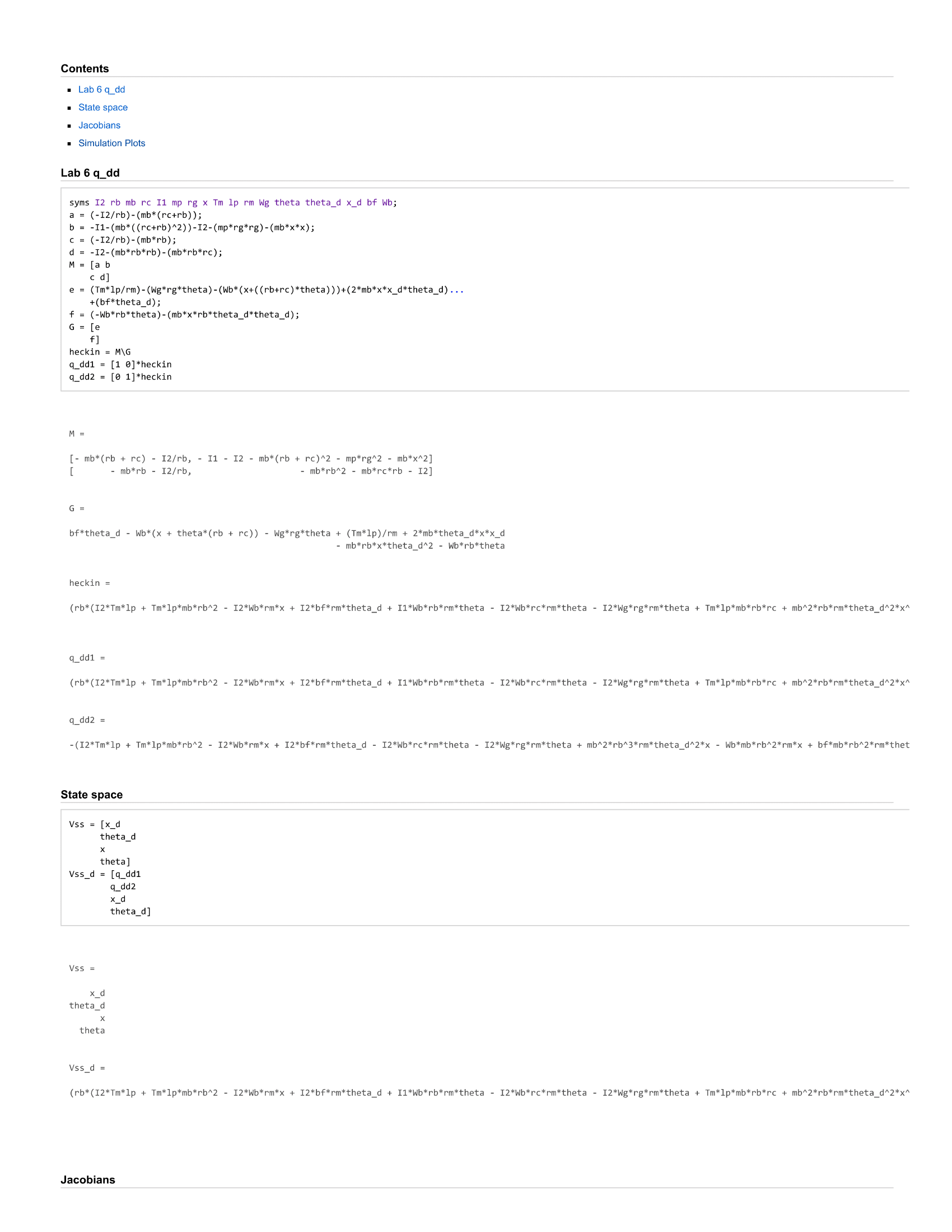
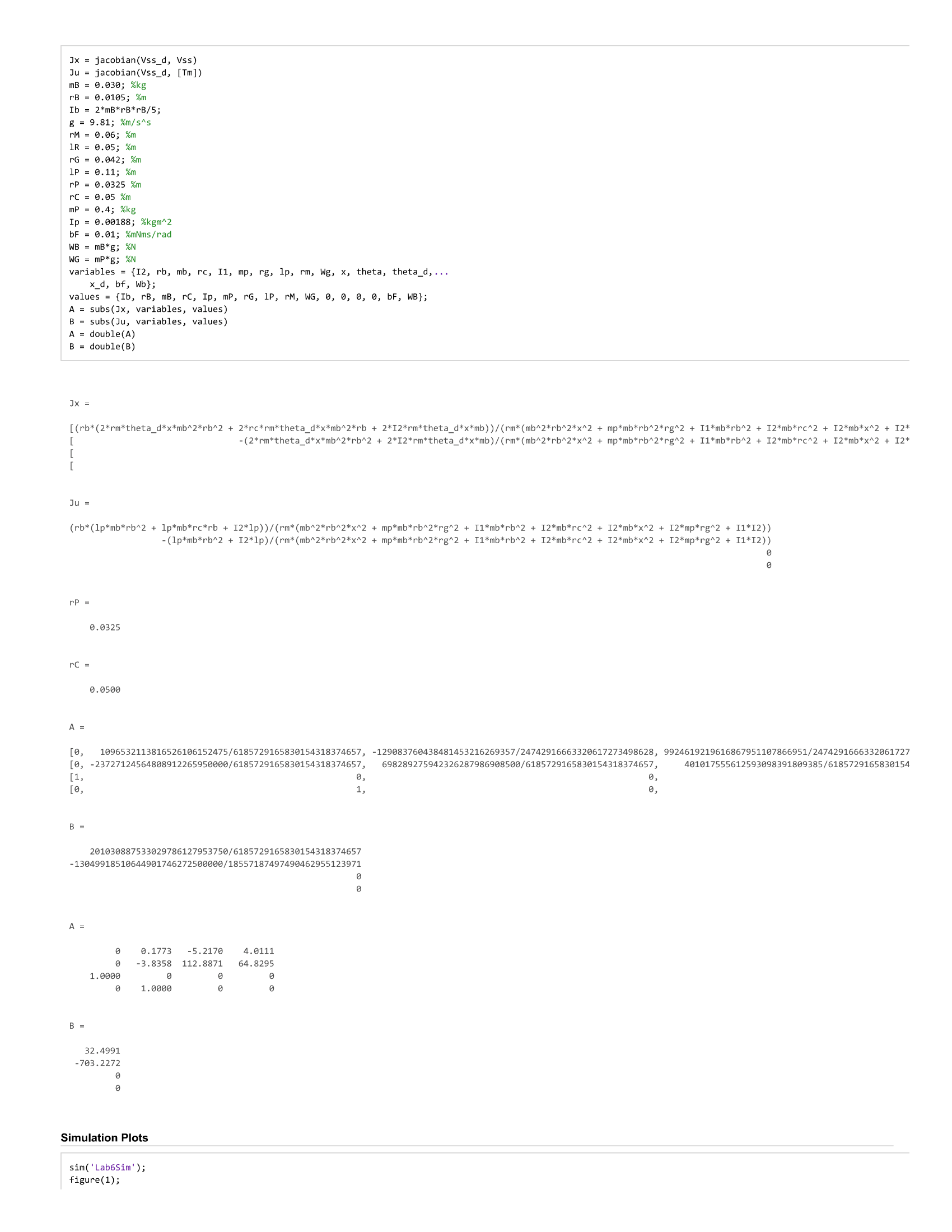
The goal of this lab was to linearize our kinematic equations from lab5 and then turn them into state space vectors.
This was done in MATLAB, and then graphs showing the time dependent response of our system were created using simulink. The lab was completed in collaboration with Hunter Morse (https://dhmorse.bitbucket.io/).
(Source: https://bitbucket.org/mediocre-code/me-405-lab/src/master/Lab6/)
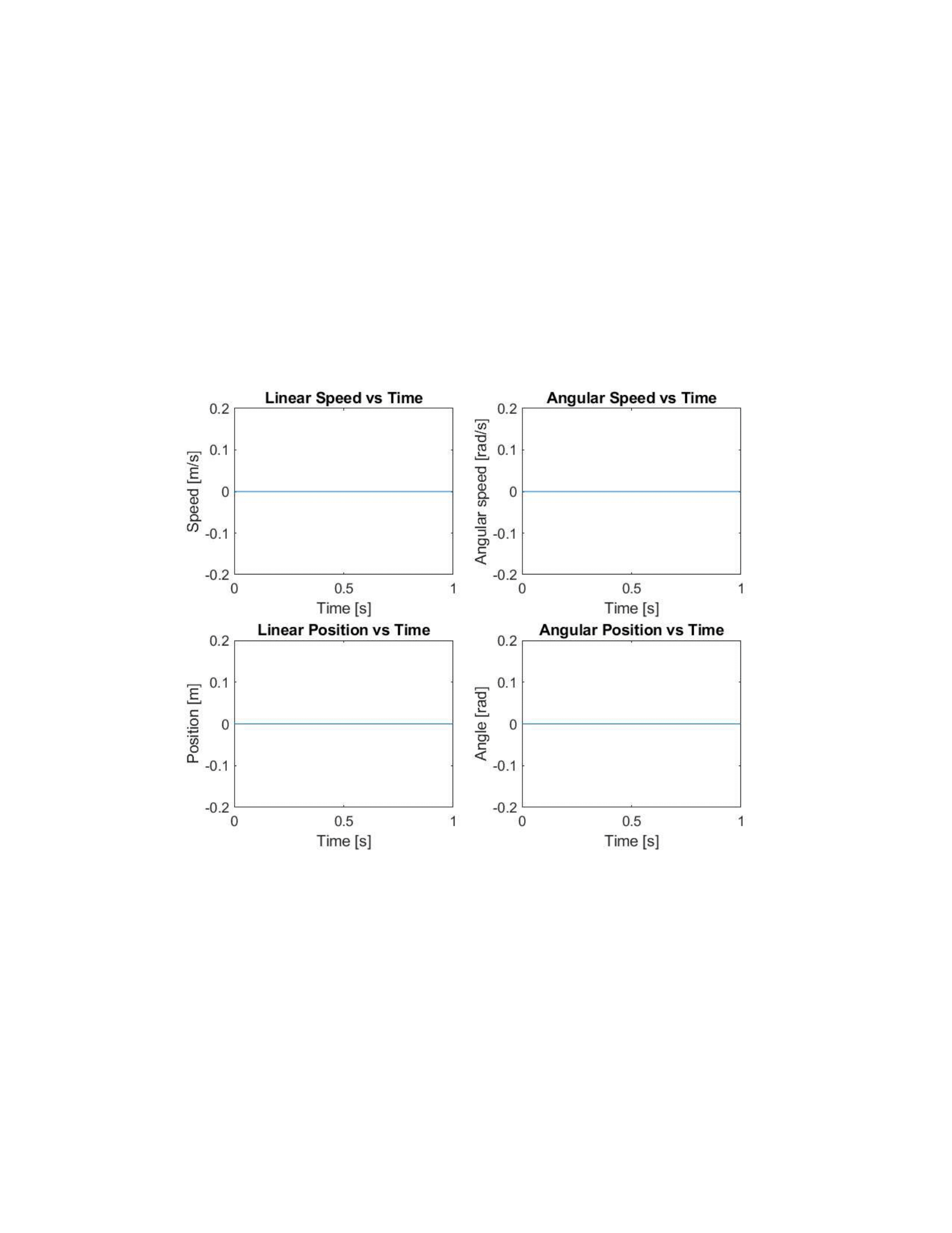
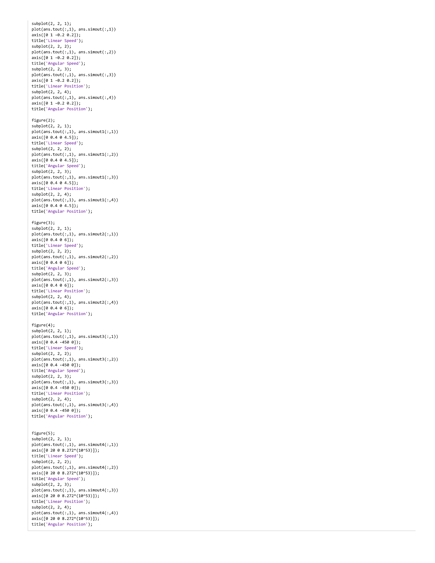
Here we can see that all four graphs show no change from their initial position. This is exactly what we would expect if a ball was placed dead center on the table while it is perfectly balanced. With all initial conditions at zero, nothing should change.
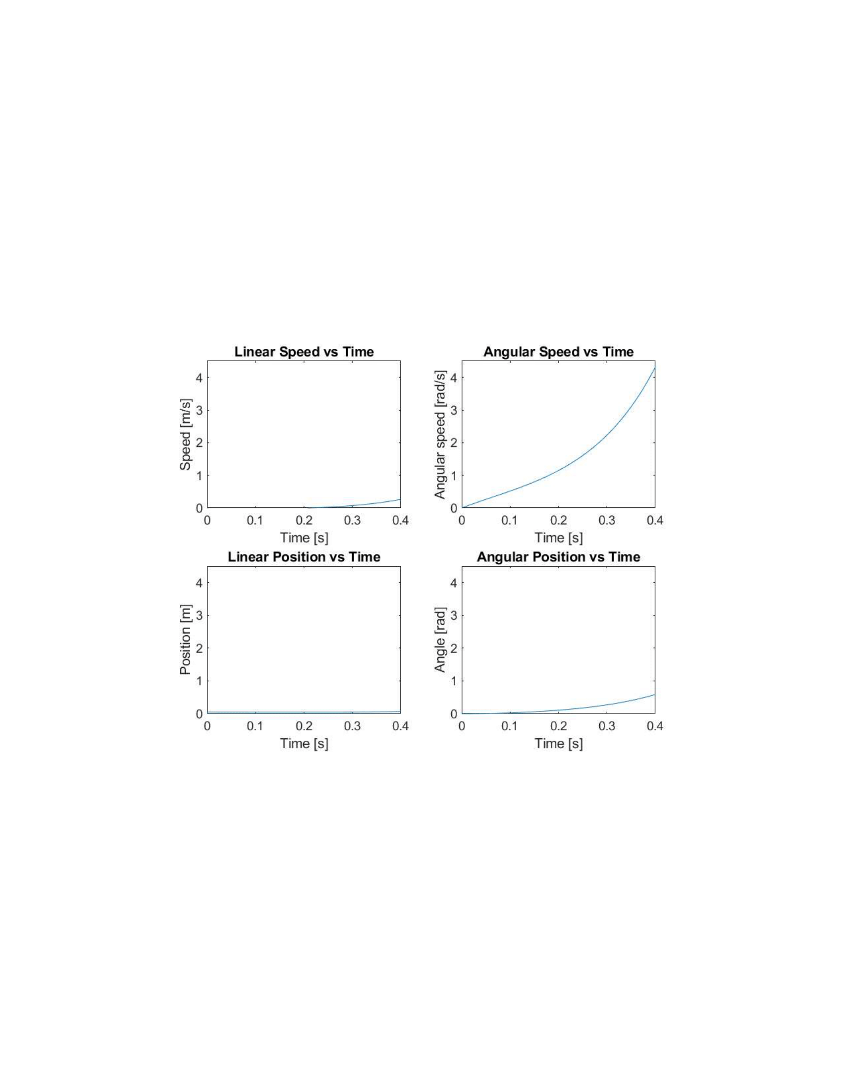
In these graphs we can see that when the ball is placed slightly offset from the center of the platform, all conditions begin to accelerate exponentially. More importantly, it is the velocities that change the most. This may seem strange, yet it actually makes sense. We are only taking data for about 0.4s, so we should not see as much change in the actual position in such a short amount of time. However, The velocity can increase dramatically in that short amount of time. As the ball pushes down on the platform, it can accelate more while also changing the angle of the platform, even without those things obviously changing much to the naked eye.
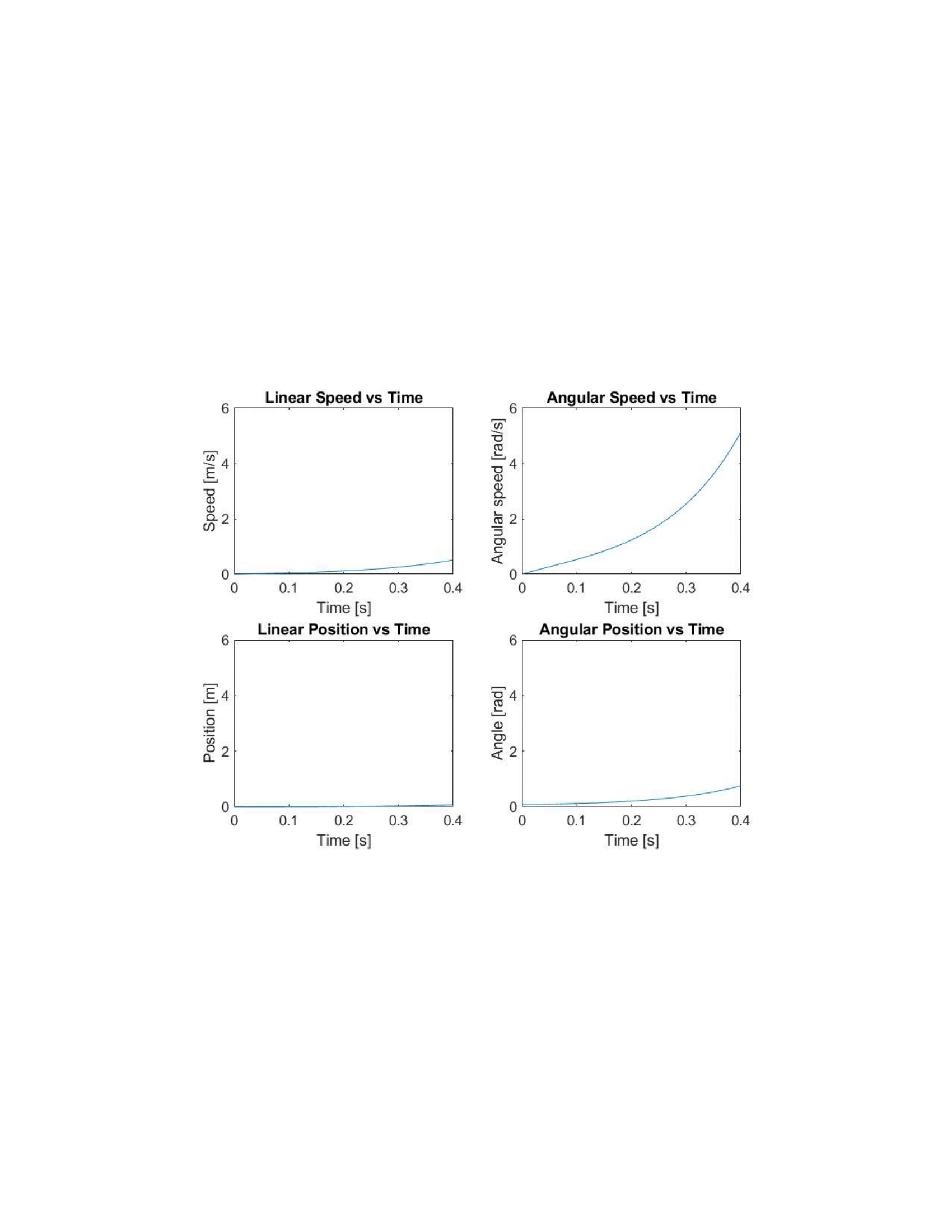
The graphs for case three show the graphs of the angular speed and position changing the most, with the linear speed close behind. Because the initial condition was an angular offset, it makes sense that it is the angles that are more affected in this case. We see that the velocity of the ball progressively increases as well, due to the effect of gravity on the ball, which in turn causes the table, already unbalanced, to tilt even faster. Thus, do to the imbalance of the initial conditions and the motion of the ball, we see the angular velocity of the table increasing more than any other graph.
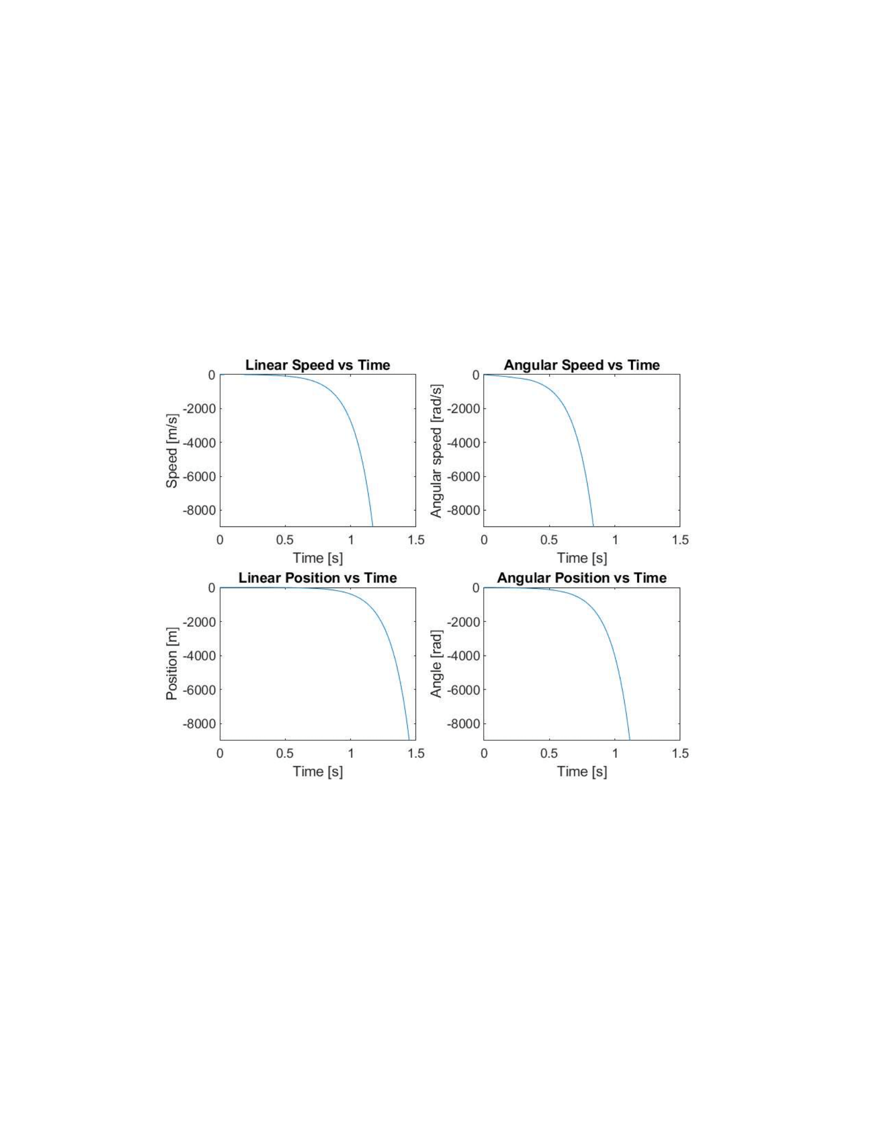
With these graphs the inition condition was an impulse to begin with. This means that the system actually starts in motion, which is a large change from the past three systems. This is why we see such a huge change in the graphs of case 4, though I did extend them to see more of the action. However, these graphs still shot away more than the others. Obviously position will be affected by the motion of the table. This large push from the table cause a lot change in position, more than we have seen before. The velocity graphs were also much larger than before. Both of these are also affected by the inertia. Because these bodies began in motion, it is "easier" for them to stay in motion. This is a major cause in the increased response.
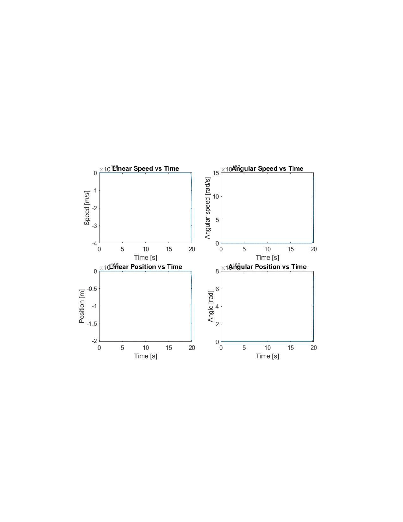
I was extremely disappointed with my results from the feedback graphs. I wanted to see the response settle back down to zero, and I was excited to see that response. I went through and double checked all my work to make sure that it was all correct. My A and B matrices were exactly the same as what Charlie gave us to check our work. I also tried re-checking my feedback loops and my initial conditions. They were still exactly what I expected them to be. To sum it up, I do not understand why my graphs are wrong. I searched for hours to find the problem, and even my work for the gains was correct, and it was based on numbers from this lab. So I cannot say what is causing them to be wrong, but I do know what they should be. These conditions of these graphs should increase, then decrease until it increases in the other direction, and repeat until it settles back down to zero. This would simulate the motion of the ball when it has an actual controller attempting to push the ball back to the origin. It will overshoot on both sides but less so with each consecutive cycle until it reaches and stays at zero. If this were an ideal system it would just go back to zero and stay there.